勤奋的凯尔森同学10000h刻意练习Day19：PyTorch入门与自动微分 —— 从张量操作到线性回归实战

所属专栏: 凯尔森的10000h刻意练习
Slogan: 一个36岁程序员,研究生(学硕),前世界500强top20软件开发Java工程师,用10000小时深耕AI,目标Top10 AI资深工程师,全程日更记录。

NumPy手搓的反向传播能用,可一旦网络深了、参数多了,谁来帮你记计算图、自动算梯度？

Day18用NumPy手搓了反向传播的每个环节。今天换上工业级工具PyTorch：它的Tensor在NumPy基础上多了GPU加速和自动微分,autograd引擎会把前向计算的每一步记成计算图,反向传播时沿图自动求导——你只管写前向,梯度交给框架。先练熟张量的创建、类型、运算、索引、形状和拼接,这些API是后面每行模型代码的地基;再用autograd跑一个完整的线性回归;最后把激活函数、全连接层和Dropout的API一次备齐。

1.1 张量创建

Tensor(张量)是PyTorch的核心数据结构。张量在不同学科中有不同的意义,在深度学习中张量表示一个多维数组,是标量、向量、矩阵的扩展。例如,一张RGB图像的数据就是一个三维张量,第1维是图像的高,第2维是图像的宽,第3维是图像的颜色通道。

1.1.1 基本张量创建

torch.tensor(data)创建指定内容的张量

import torch
import numpy as np

# 创建标量张量
tensor1 = torch.tensor(10)
print(tensor1)

# 使用列表创建张量
tensor2 = torch.tensor([1, 2, 3])
print(tensor2)

# 使用numpy创建张量
tensor3 = torch.tensor(np.array([[1, 2, 3], [4, 5, 6], [7, 8, 9]]))
print(tensor3)

torch.Tensor(size)创建指定形状的张量

import torch

# 创建指定形状的张量,默认类型为float32
tensor1 = torch.Tensor(3, 2, 4)
print(tensor1)
print(tensor1.dtype)

# 也可以用来创建指定内容的张量
tensor2 = torch.Tensor([[1, 2, 3, 4], [5, 6, 7, 8]])
print(tensor2)

创建指定类型的张量

可通过torch.IntTensor()、torch.FloatTensor()等创建。

或在torch.tensor()中通过dtype参数指定类型。

import torch

# 创建int32类型的张量
tensor1 = torch.IntTensor(2, 3)
tensor2 = torch.tensor([1, 2, 3], dtype=torch.int32)
print(tensor1)
print(tensor2)

# 元素类型不匹配则会进行类型转换
tensor1 = torch.IntTensor([1.1, 2.2, 3.6])
tensor2 = torch.tensor([3.1, 2.2, 1.6], dtype=torch.int32)
print(tensor1)
print(tensor2)

# 创建int64类型的张量
tensor1 = torch.LongTensor([1, 2, 3])
tensor2 = torch.tensor([1, 2, 3], dtype=torch.int64)
print(tensor1, tensor1.dtype)
print(tensor2, tensor1.dtype)

# 创建int16类型的张量
tensor1 = torch.ShortTensor(2, 2)
tensor2 = torch.tensor([1, 2, 3], dtype=torch.int16)
print(tensor1, tensor1.dtype)
print(tensor2, tensor1.dtype)

# 创建float32类型的张量
tensor1 = torch.FloatTensor([9, 8, 7])
tensor2 = torch.tensor([1, 2, 3], dtype=torch.float32)
print(tensor1, tensor1.dtype)
print(tensor2, tensor1.dtype)

# 创建float64类型的张量
tensor1 = torch.DoubleTensor(2, 3, 1)
tensor2 = torch.tensor([1, 2, 3], dtype=torch.float64)
print(tensor1)
print(tensor2)

1.1.2 指定区间的张量创建

torch.arange(start, end, step)在区间内按步长创建张量

import torch

# torch.arange(start, end, step) 在区间[start,end)中创建步长为step的张量
tensor1 = torch.arange(10, 30, 2)
print(tensor1)

# torch.arange(end) 创建区间为[0,end),步长为1的张量
tensor2 = torch.arange(6)
print(tensor2)

torch.linspace(start, end, steps)在区间内按元素数量创建张量

import torch

# torch.linspace(start, end, steps) 在区间按元素数量创建张量
tensor1 = torch.linspace(10, 30, 5)
print(tensor1)

torch.logspace(start, end, steps, base)在指数区间内按指定底数创建张量

import torch

# torch.logspace(start, end, steps, base) 在区间[start,end]之间生成steps个数,并以base为底,区间内的数为指数创建张量
tensor1 = torch.logspace(1, 3, 3, 2)
print(tensor1)

1.1.3 按数值填充张量

• torch.zeros(size)创建指定形状的全0张量

• torch.ones(size)创建指定形状的全1张量

• torch.full(size, value)创建指定形状的按指定值填充的张量

• torch.empty(size)创建指定形状的未初始化的张量

• torch.zeros_like(input)创建与给定张量形状相同的全0张量

• torch.ones_like(input)创建与给定张量形状相同的全1张量

• torch.full_like(input, value)创建与给定张量形状相同的按指定值填充的张量

• torch.empty_like(input)创建与给定张量形状相同的未初始化的张量

import torch

# torch.zeros(size) 创建指定形状的全0张量
tensor1 = torch.zeros(2, 3)
print(tensor1)

# torch.ones_like(input) 创建与给定张量形状相同的全1张量
tensor2 = torch.ones_like(tensor1)
print(tensor2)

# torch.full(size,fill_value) 创建指定形状的按指定值填充的张量
tensor1 = torch.full((2, 3), 6)
print(tensor1)

# torch.empty_like(input) 创建与给定张量形状相同的未初始化的张量
tensor2 = torch.empty_like(tensor1)
print(tensor2)

• torch.eye(n, [m])创建单位矩阵

import torch

# torch.eye(n) 创建n*n的单位矩阵
tensor1 = torch.eye(3)
print(tensor1)

# torch.eye(n, m) 按指定的行和列创建
tensor2 = torch.eye(3, 4)
print(tensor2)

1.1.4 随机张量创建

• torch.rand(size)创建在[0,1)上均匀分布的,指定形状的张量

• torch.randint(low, high, size)创建在[low,high)上均匀分布的,指定形状的张量

• torch.randn(size)创建标准正态分布的,指定形状的张量

• torch.normal(mean,std,size)创建自定义正态分布的,指定形状的张量

• torch.rand_like(input)创建在[0,1)上均匀分布的,与给定张量形状相同的张量

• torch.randint_like(input, low, high)创建在[low,high)上均匀分布的,与给定张量形状相同的张量

• torch.randn_like(input)创建标准正态分布的,与给定张量形状相同的张量

import torch

# torch.rand(size) 创建在[0,1)上均匀分布的,指定形状的张量
tensor1 = torch.rand(2, 3)
print(tensor1)

# torch.rand_like(input) 创建在[0,1)上均匀分布的,与给定张量形状相同的张量
tensor2 = torch.randint_like(tensor1, 1, 10)
print(tensor2)

# torch.randn(size) 创建标准正态分布的,指定形状的张量
tensor1 = torch.randn(4, 2)
print(tensor1)

# torch.normal(mean,std,size) 创建自定义正态分布的,指定形状的张量。mean为均值,std为标准差
tensor2 = torch.normal(5, 1, tensor1.shape)
print(tensor2)

• torch.randperm(n)生成从0到n-1的随机排列,类似洗牌

import torch

# torch.randperm(n) 生成从0到n-1的随机排列
tensor1 = torch.randperm(10)
print(tensor1)

• torch.random.initial_seed()查看随机数种子

• torch.manual_seed(seed)设置随机数种子

import torch

# 查看随机数种子
print(torch.random.initial_seed())
# 设置随机数种子
torch.manual_seed(42)
print(torch.random.initial_seed())

1.2 张量类型转换与NumPy互操作

1.2.1 张量元素类型转换

为什么要做类型转换？PyTorch的CUDA内核主要针对float32(以及float16/bfloat16)优化,整型张量或float64放到GPU上要么直接报错、要么退回CPU慢速执行;另外autograd只能对浮点张量求导,整型是无法反向传播的。所以把数据送进模型前,通常要先把整型特征转成float32,这也是后面线性回归、神经网络里所有参数默认float32的原因。float16/bfloat16常用于混合精度训练以省显存、提速度,但float16数值范围小、需要配合损失缩放(loss scaling),初学阶段先用float32最稳妥。

Tensor.type(dtype)修改张量的类型

import torch

tensor1 = torch.tensor([1, 2, 3])
print(tensor1, tensor1.dtype)

# 使用type方法修改张量的类型
tensor1 = tensor1.type(torch.float32)
print(tensor1, tensor1.dtype)

Tensor.double()等修改张量的类型

import torch

tensor1 = torch.tensor([1, 2, 3])
print(tensor1, tensor1.dtype)

# 使用double方法修改张量的类型
tensor1 = tensor1.double()
print(tensor1)
# 使用long方法修改张量的类型
tensor1 = tensor1.long()
print(tensor1, tensor1.dtype)

1.2.2 Tensor与ndarray转换

Tensor.numpy()将Tensor转换为ndarray,共享内存。使用copy()避免共享内存

import torch

# 使用numpy()方法将Tensor转换为ndarray,共享内存
tensor1 = torch.rand(3, 2)
numpy_array = tensor1.numpy()
print(tensor1)
print(numpy_array)
print(type(tensor1), type(numpy_array))
print()
tensor1[:, 0] = 4
print(tensor1)
print(numpy_array)
print()

# 使用copy()方法避免共享内存
numpy_array = tensor1.numpy().copy()
tensor1[:, 0] = -1
print(tensor1)
print(numpy_array)

torch.from_numpy(ndarray)将ndarray转换为Tensor,共享内存。使用copy()避免共享内存

import torch
import numpy as np

# 使用from_numpy()方法将ndarray转换为Tensor,共享内存
numpy_array = np.random.randn(3)
tensor1 = torch.from_numpy(numpy_array)
print(numpy_array)
print(tensor1)
print()
numpy_array[0] = 100
print(numpy_array)
print(tensor1)
print()

# 使用copy()方法避免共享内存
tensor1 = torch.from_numpy(numpy_array.copy())
numpy_array[0] = -1
print(numpy_array)
print(tensor1)

torch.tensor(ndarray)将ndarray转换为Tensor,不共享内存

import torch
import numpy as np

# 使用torch.tensor()将ndarray转换为Tensor
numpy_array = np.random.randn(3)
tensor1 = torch.tensor(numpy_array)
print(numpy_array)
print(tensor1)
print()
numpy_array[0] = 100
print(numpy_array)
print(tensor1)

1.2.3 Tensor与标量转换

若张量中只有1个元素,Tensor.item()可提取张量中元素为标量。

import torch

tensor1 = torch.tensor(1)

print(tensor1)

print(tensor1.item())

1.3 张量数值计算

1.3.1 基本运算

四则运算

• +、-、*、/加减乘除

• add()、sub()、mul()、div()加减乘除,不改变原数据

• add_()、sub_()、mul_()、div_()加减乘除、修改原数据

import torch

tensor1 = torch.randint(1, 9, (2, 3))
print(tensor1)
print(tensor1 + 10)
print()

# add(),不修改原数据
print(tensor1.add(10))
print(tensor1)
print()

# add_(),修改原数据
print(tensor1.add_(10))
print(tensor1)

-、neg()、neg_()取负

import torch

tensor1 = torch.tensor([1, 2, 3])
print(-tensor1)
print()

print(tensor1.neg())
print(tensor1)
print()

print(tensor1.neg_())
print(tensor1)

**、pow()、pow_()求幂

import torch

tensor1 = torch.tensor([1, 2, 3])
print(tensor1**2)
print()

print(tensor1.pow(2))
print(tensor1)
print()

print(tensor1.pow_(2))
print(tensor1)

sqrt()、sqrt_()求平方根

import torch

tensor1 = torch.tensor([1.0, 2.0, 3.0])
print(tensor1.sqrt())
print(tensor1)
print()

print(tensor1.sqrt_())
print(tensor1)

exp()、exp_()以e为底数求幂

import torch

tensor1 = torch.tensor([1.0, 2.0, 3.0])
print(2.71828183**tensor1)
print()

print(tensor1.exp())
print(tensor1)
print()

print(tensor1.exp_())
print(tensor1)

log()、log_()以e为底求对数

import torch

tensor1 = torch.tensor([1.0, 2.0, 3.0])
print(tensor1.log())
print(tensor1)
print()

print(tensor1.log_())
print(tensor1)

1.3.2 哈达玛积(元素级乘法)

两个矩阵对应位置元素相乘称为哈达玛积(Hadamard product)。

使用*、mul()实现两个形状相同的张量之间对位相乘。

import torch

tensor1 = torch.tensor([[1, 2], [3, 4]])
tensor2 = torch.tensor([[1, 2], [3, 4]])
print(tensor1 * tensor2)
print(tensor1.mul(tensor2))

1.3.3 矩阵乘法运算

mm()严格用于二维矩阵相乘。

@、matmul()支持多维张量,按最后两个维度做矩阵乘法,其他维度相同,或者至少一个张量对应维度为1,广播后进行运算。

import torch

# 2维矩阵的矩阵乘法
tensor1 = torch.tensor([[1, 2, 3], [4, 5, 6]])
tensor2 = torch.tensor([[1, 2], [3, 4], [5, 6]])
print(tensor1)
print(tensor2)
print(tensor1.mm(tensor2))
print(tensor1 @ tensor2)
print(tensor1.matmul(tensor2))
print()

# 3维张量的矩阵乘法
tensor1 = torch.tensor([[[1, 2, 3], [4, 5, 6]], [[6, 5, 4], [3, 2, 1]]])
tensor2 = torch.tensor([[[1, 2], [3, 4], [5, 6]], [[6, 5], [4, 3], [2, 1]]])
print(tensor1)
print(tensor2)
print(tensor1 @ tensor2)
print(tensor1.matmul(tensor2))

1.3.4 节省内存

运行一些操作时可能为新结果分配内存,例如执行X=X@Y后会发现id(X)变了,这是因为Python先计算X@Y并为结果分配新内存,再让X指向这块新内存。

import torch

X = torch.randint(1, 9, (3, 2, 4))
Y = torch.randint(1, 9, (3, 4, 1))
print(id(X))
X = X @ Y
print(id(X), end="\n\n")

# 如果后续X不再重复使用,可以使用X[:] = X @ Y来减少内存开销。
X = torch.randint(1, 9, (3, 2, 4))
Y = torch.randint(1, 9, (3, 4, 1))
print(id(X))
X[:] = X @ Y
print(id(X))

1.4 张量运算函数:一把梭的统计工具箱

常见运算函数：

sum()求和

mean()求均值

max()/min()求最大/最小值及其索引

argmax()/argmin()求最大值/最小值的索引

std()求标准差

unique()去重

sort()排序

import torch

tensor1 = torch.randint(1, 9, (3, 2, 4))
tensor1 = tensor1.float()
print(tensor1)
print()

# sum() 求和
print("求和")
print(tensor1.sum())
print("按第0个维度求和")
print(tensor1.sum(dim=0))
print()

# mean() 求均值
print("求均值")
print(tensor1.mean())
print("按第1个维度求均值")
print(tensor1.mean(dim=1))
print()

# max() 求最大值
print("求最大值")
print(tensor1.max())
print("按第2个维度求最大值与索引")
print(tensor1.max(dim=2))
print()

# argmin() 求最小值索引
print("求最小值索引")
print(tensor1.argmin())
print()

# std() 求标准差
print("求标准差")
print(tensor1.std())
print()

# unique() 去重
print("去重")
print(tensor1.unique())
print()

# sort() 排序
print("排序")
print(tensor1.sort())

1.5 张量索引操作:精确制导的元素定位

#简单索引
import torch

tensor1 = torch.randint(1, 9, (3, 5, 4))
print(tensor1)
print()

# 取 第0维第0
print(tensor1[0])
print()

# 取 第0维所有,第1维第1
print(tensor1[:, 1])
print()

# 取 第0维第2,第1维第1,第2维第3
print(tensor1[2, 1, 3])


#范围索引
tensor1 = torch.randint(1, 9, (3, 5, 4))
print(tensor1)
print()

# 取 第0维第1到最后
print(tensor1[1:])
print()

# 取 第0维最后,第1维1到3(包含3),第2维0到2(包含2)
print(tensor1[-1:, 1:4, 0:3])
print()


#列表索引
tensor1 = torch.randint(1, 9, (3, 5, 4))
print(tensor1)
print()

# 取 第0维第0,第1维第1 和 第0维第1,第1维第2
print(tensor1[[0, 1], [1, 2]])
print()

# 取 第0维第0,第1维第1、2 和 第0维第1,第1维第1、2
print(tensor1[[[0], [1]], [1, 2]])


#布尔索引
tensor1 = torch.randint(1, 9, (3, 5, 4))
print(tensor1)
print()

# 取 第2维第0大于5的,返回(dim0,dim1)形状的索引
print(tensor1[:, :, 0] > 5)
print(tensor1[tensor1[:, :, 0] > 5])
print()

# 取 第1维第1大于5的,返回(dim0,dim2)形状的索引
mask = tensor1[:, 1, :] > 5
print(mask)
tensor2 = tensor1.permute(0, 2, 1)  # 转换维度为(dim0,dim2,dim1)
print(tensor2[mask])
tensor2 = tensor2[mask].permute(1, 0)  # 转换维度为(dim1,?)
print(tensor2)
print()

# 取 第1维第1,第2维第2大于5的,返回(dim0)形状的索引
print(tensor1[:, 1, 2] > 5)
print(tensor1[tensor1[:, 1, 2] > 5])

1.6 张量形状操作:数据的自由塑形

import torch
#交换维度
#transpose()交换两个维度

tensor1 = torch.randint(1, 9, (2, 3, 6))
print(tensor1)
print(tensor1.transpose(1, 2))  # 交换第1维和第2维

#permute()重新排列多个维度
tensor1 = torch.randint(1, 9, (2, 3, 6))
print(tensor1)
print(tensor1.permute(2, 0, 1))  # (2, 3, 6)->(6, 2, 3)


#调整形状
#reshape()调整张量的形状
tensor1 = torch.randint(1, 9, (3, 5, 4))
print(tensor1)
print(tensor1.reshape(6, 10))
print(tensor1.reshape(3, -1))


#view()调整张量的形状,需要内存连续。共享内存
#is_contiguous()判断是否内存连续
#contiguous()转换为内存连续
tensor1 = torch.randint(1, 9, (3, 5, 4))
print(tensor1)
print(tensor1.is_contiguous())  # is_contiguous()判断是否内存连续
print(tensor1.view(-1, 10))

tensor1 = tensor1.T
print(tensor1.is_contiguous())  # is_contiguous()判断是否内存连续
print(tensor1.contiguous().view(-1))  # contiguous()强制内存连续


#增加或删除维度
#unsqueeze()在指定维度上增加1个维度
tensor1 = torch.tensor([1, 2, 3, 4, 5])
print(tensor1)
# 在0维上增加一个维度
print(tensor1.unsqueeze(dim=0))
# 在1维上增加一个维度
print(tensor1.unsqueeze(dim=1))
# 在-1维上增加一个维度
print(tensor1.unsqueeze(dim=-1))


#squeeze()删除大小为1的维度
tensor1 = torch.tensor([1, 2, 3, 4, 5])
print(tensor1.unsqueeze_(dim=0))
print(tensor1.squeeze())

1.7 张量拼接操作:cat与stack

import torch
#torch.cat()张量拼接,按已有维度拼接。除拼接维度外,其他维度大小须相同
tensor1 = torch.randint(1, 9, (2, 2, 5))
tensor2 = torch.randint(1, 9, (2, 1, 5))
print(tensor1)
print(tensor2)
print(torch.cat([tensor1, tensor2], dim=1))


#torch.stack()张量堆叠,按新维度堆叠。所有张量形状必须一致
torch.manual_seed(42)
tensor1 = torch.randint(1, 9, (3, 1, 5))
tensor2 = torch.randint(1, 9, (3, 1, 5))
print(tensor1)
print(tensor2)
tensor3 = torch.stack([tensor1, tensor2], dim=2)
print(tensor3)
print(tensor3.shape)

1.8 自动微分模块:计算图与梯度的自动计算

前7节把张量的创建、运算、索引、形状、拼接都练熟了,但这只解决了"怎么算"的问题。训练神经网络还需要"怎么学"——即怎么拿到损失对每个参数的梯度。Day18用NumPy手推链式法则,一旦网络加深就力不从心。这一节换用PyTorch的autograd：你只管写前向,框架帮你记图、帮你求导。

1.8.1 计算图:神经网络训练的账本

训练神经网络时,框架会根据设计好的模型构建一个计算图(computational graph),来跟踪计算是哪些数据通过哪些操作组合起来产生输出,并通过反向传播算法,根据损失函数对参数的梯度来调整参数(模型权重)。

PyTorch具有一个内置的微分引擎torch.autograd,用于支持计算图中梯度的自动计算。

为什么"前向记录+反向沿图"就能自动算出梯度？关键在于每个算子只负责自己那一小段导数。前向时,PyTorch每执行一个运算(乘法、加法、激活),就把"这个运算的输入值"和"这个运算的局部导数怎么算"打包成一个grad_fn挂在结果张量上,节点之间用指针连成一张有向无环图。反向时,从损失(根节点)出发,沿着指针反向走,每到一处就把该节点的局部导数和上游传回来的梯度相乘——这正是链式法则$\frac{\partial L}{\partial w}=\frac{\partial L}{\partial z}\cdot \frac{\partial z}{\partial w}$的机械执行。换句话说,autograd不需要懂你的整体公式长什么样,它只把无数个"本地小导数"按图连乘,自动拼出任意复杂函数的梯度。这也是为什么写前向时只要用PyTorch的运算,反向就能"免费"得到。

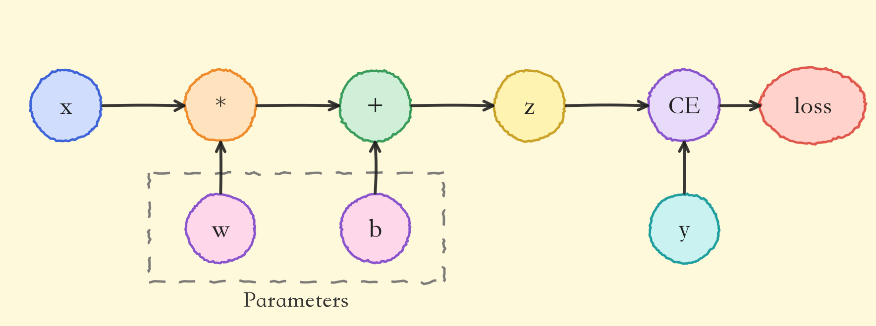
考虑最简单的单层神经网络,具有输入x、参数w、偏置b以及损失函数：

1.8.2 最小单层神经网络实战:一次前向+一次反向

import torch

# 输入x
x = torch.tensor(10.0)
# 目标值y
y = torch.tensor(3.0)

# 初始化权重w
w = torch.rand(1, 1, requires_grad=True)
# 初始化偏置b
b = torch.rand(1, 1, requires_grad=True)
z = w * x + b
# 设置损失函数
loss = torch.nn.MSELoss()
loss_value = loss(z, y)
# 反向传播
loss_value.backward()
# 打印w,b的梯度
print("w的梯度:\n", w.grad)
print("b的梯度:\n", b.grad)

整个流程就五步：定义叶子节点→前向算出z→算损失→backward()反向传播→从.grad属性读梯度。Day18手推半天的链式法则,这里一行backward()搞定。

1.8.3 叶子节点:计算图的基石

该计算图中x、w、b为叶子节点,即最基础的节点。叶子节点的数据并非由计算生成,因此是整个计算图的基石,叶子节点张量不能执行in-place操作。而最终的loss为根节点。

可通过is_leaf属性查看张量是否为叶子节点：

print(x.is_leaf)  # True
print(w.is_leaf)  # True
print(b.is_leaf)  # True
print(z.is_leaf)  # False
print(y.is_leaf)  # True
print(loss_value.is_leaf)  # False

z和loss_value是计算出来的,所以不是叶子节点;x、w、b、y是手动创建的,是叶子节点。

1.8.4 数据与运算的记录:data与grad_fn

自动微分的关键就是记录节点的数据与运算。数据记录在张量的data属性中,计算记录在张量的grad_fn属性中。具体地说,grad_fn指向"创建这个张量的那个运算"的反向函数——也就是该运算的局部导数配方。例如z = w * x + b里的z,它的grad_fn指向加法运算的反向函数,加法又链到乘法的反向函数。反向传播时,autograd就是顺着这些grad_fn指针,把每一步的局部导数一路乘回叶子节点。而requires_grad是一个开关：设为True表示"请追踪这个张量上的所有运算,将来我要对它求梯度"。模型参数默认requires_grad=True,输入数据通常为False——只对需要优化的参数建图求导,省内存也省算力。

计算图根据搭建方式可分为静态图和动态图。静态图(如早期TensorFlow)需要先用代码声明整张图再喂数据运行,图一旦建好便不易改动;动态图(PyTorch采用)则是边运行边建图,每跑一次前向就即时构造一张新图,自然支持条件分支和循环。PyTorch在计算的过程中逐步搭建计算图,同时对每个Tensor都存储grad_fn供自动微分使用。这也是PyTorch比早期TensorFlow静态图更好调试的原因——图就是代码跑出来的,断点想打哪打哪。

1.8.5 requires_grad、梯度的释放与累积

若设置张量参数requires_grad=True,则PyTorch会追踪所有基于该张量的操作,并在反向传播时计算其梯度。依赖于叶子节点的节点,requires_grad默认为True。当计算到根节点后,在根节点调用backward()方法即可通过反向传播计算出计算图中所有节点的梯度。

非叶子节点的梯度在反向传播之后会被释放掉(除非设置参数retain_grad=True)。而叶子节点的梯度在反向传播之后会保留(累积)。通常需要使用optimizer.zero_grad()清零参数的梯度。

这条规则直接关系到训练循环的写法：每个batch都要先zero_grad()再backward(),否则梯度会一轮轮累加,越训越歪——这是新手最常踩的坑。

1.8.6 detach:把变量移出计算图

为什么需要把变量移出计算图？因为有些下游用途根本不该往回传梯度：比如训练中要打印当前loss的数值、把中间特征拿去画图或算准确率,或者像GAN里用一个网络的部分输出当标签去训练另一个网络。如果让梯度沿这些分支继续回传,要么污染参数更新、要么白算一堆没用的梯度。Tensor.detach()返回一个与原张量同值的新张量,但切断它和计算图的连接——它的grad_fn为None,requires_grad为False,梯度不会再从它流回原计算图。

import torch

x = torch.ones(2, 2, requires_grad=True)
y = x * x
# 分离y来返回一个新变量u
u = y.detach()
z = u * x
# 梯度不会向后流经u到x
z.sum().backward()
# 反向传播函数计算z=u*x关于x的偏导数时将u作为常数处理,而不是z=x*x*x关于x的偏导数
x.grad == u
# tensor([[True, True],
#         [True, True]])

detach的典型用途：截断梯度流(比如RNN的截断反向传播,避免序列过长导致梯度爆炸/消失和显存炸掉)、把带梯度的张量转成纯数据去画图或算指标。

和detach成对出现的还有torch.no_grad()：它是一个上下文管理器(也可作装饰器),进入with torch.no_grad():块后,框架整段都不再记录运算、不建计算图。detach是"切掉一个张量",no_grad是"关掉一整片代码的追踪"。在做纯推理或算验证指标时,用torch.no_grad()包起来,既省显存又跑得更快——Day20的验证循环里就会看到它。

1.9 机器学习案例:线性回归

理论讲完,立刻上手一个完整项目。通过PyTorch训练一个模型一般分为以下4个步骤：

准备数据 → 构建模型 → 定义损失函数与优化器 → 模型训练

接下来,构建数据集并使用PyTorch实现线性回归：

import torch
import matplotlib.pyplot as plt
from torch import nn, optim  # 模型、损失函数和优化器
from torch.utils.data import TensorDataset, DataLoader  # 数据集和数据加载器

# 构建数据集
X = torch.randn(100, 1)  # 输入
w = torch.tensor([2.5])  # 权重
b = torch.tensor([5.2])  # 偏置
noise = torch.randn(100, 1) * 0.1  # 噪声
y = w * X + b + noise  # 目标
dataset = TensorDataset(X, y)  # 构造数据集对象
dataloader = DataLoader(
    dataset, batch_size=10, shuffle=True
)  # 构造数据加载器对象,batch_size为每次训练的样本数,shuffle为是否打乱数据

# 构造模型
model = nn.Linear(in_features=1, out_features=1)  # 线性回归模型,1个输入,1个输出

# 损失函数和优化器
loss = nn.MSELoss()  # 均方误差损失函数
optimizer = optim.SGD(model.parameters(), lr=1e-3)  # 随机梯度下降,学习率0.001

# 模型训练
loss_list = []
for epoch in range(1000):
    total_loss = 0
    train_num = 0
    for x_train, y_train in dataloader:
        # 每次训练一个batch大小的数据
        y_pred = model(x_train)  # 模型预测
        loss_value = loss(y_pred, y_train)  # 计算损失
        total_loss += loss_value.item()
        train_num += len(y_train)
        optimizer.zero_grad()  # 梯度清零
        loss_value.backward()  # 反向传播
        optimizer.step()  # 更新参数
    loss_list.append(total_loss / train_num)

print(model.weight, model.bias)  # 打印权重和偏置
plt.plot(loss_list)
plt.xlabel("epoch")
plt.ylabel("loss")
plt.show()

这段代码是PyTorch训练的标准模板,值得逐行吃透：

• 数据：TensorDataset把X和y打包成数据集,DataLoader负责按batch切分和打乱(相比Day18在NumPy里手写循环遍历样本,这里切分、打乱、取batch的活全交给框架)——真实数据是$w=2.5$、$b=5.2$加一点噪声
• 模型：nn.Linear(1, 1)就是一个$y=wx+b$的线性层,w和b是它的参数
• 训练循环三件套：zero_grad()清零梯度→backward()反向传播→step()更新参数,顺序不能乱
• 结果：训练结束后model.weight会逼近2.5、model.bias会逼近5.2,损失曲线一路下降

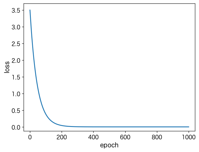
那autograd在这段代码里到底替我们算了什么？把模型展开看一眼。nn.Linear(1, 1)做的就是$\hat{y}=wx+b$,其中$w$、$b$是待学参数;MSELoss默认对batch取平均,设batch大小为$n$,第$i$个样本的残差$r_i=w{x}_i+b-y_i$,则损失为：

$$L=\frac{1}{n}\sum _{i=1}^n(w{x}_i+b-y_i{)}^2=\frac{1}{n}\sum _{i=1}^n{r}_i^2$$

对$w$求导,按链式法则从外向内一层层剥：$r_i$对$w$的偏导数$\frac{\partial r_i}{\partial w}=x_i$,先对$r_i^2$求导得$2r_i$,再乘$\frac{\partial r_i}{\partial w}$：

$$\frac{\partial L}{\partial w}=\frac{1}{n}\sum _{i=1}^{n}2r_i\cdot \frac{\partial r_i}{\partial w}=\frac{2}{n}\sum _{i=1}^n(w{x}_i+b-y_i)x_i$$

同理$r_i$对$b$的导数是1,所以：

$$\frac{\partial L}{\partial b}=\frac{2}{n}\sum _{i=1}^n(w{x}_i+b-y_i)$$

loss_value.backward()做的事情,就是沿计算图把上面这两个梯度算出来,写进model.weight.grad和model.bias.grad;optimizer.step()再按$w\leftarrow w-\eta \frac{\partial L}{\partial w}$、$b\leftarrow b-\eta \frac{\partial L}{\partial b}$更新参数(其中$\eta$是学习率)。注意代码里根本没有写任何求导公式——这一串链式法则全由autograd沿计算图自动完成,这就是自动微分的威力。

1.10 激活函数:PyTorch API速查与autograd验证

激活函数的家族成员(Sigmoid/Tanh/ReLU/Leaky ReLU/PReLU/Softmax的公式、输出区间、导数和梯度消失问题)Day16已经系统讲过,这里不再重复公式,只解决两个工程问题：PyTorch里叫什么名字、怎么验证背过的导数公式是对的。

1.10.1 API速查表

激活函数	函数式调用	层方式(nn.)	典型位置
Sigmoid	torch.sigmoid(x)	nn.Sigmoid()	二分类输出层
Tanh	torch.tanh(x)	nn.Tanh()	浅层隐藏层
ReLU	torch.relu(x)	nn.ReLU()	隐藏层默认首选
Leaky ReLU	nn.functional.leaky_relu(x, negative_slope=0.01)	nn.LeakyReLU(0.01)	ReLU"死神经元"严重时
Softmax	torch.softmax(x, dim=1)	nn.Softmax(dim=1)	多分类取概率(注意下方规则)

重要规则(Day20还会强调)： 多分类训练时模型输出层不要手动套Softmax——nn.CrossEntropyLoss内部已包含Softmax且数值更稳定。只有在预测/展示概率时才显式调用torch.softmax。

1.10.2 用autograd给Day16的导数公式做"实验验证"

Day16我们是用手推导数、NumPy画曲线的。今天有了autograd,导数曲线可以让框架算：构造requires_grad=True的x,前向算激活值,sum().backward()后直接从x.grad读出每个点的导数——一行解析公式都不用写。三个激活函数放一张图里对比：

import torch
import matplotlib.pyplot as plt

def curve_with_grad(fn, xlim):
    x = torch.linspace(xlim[0], xlim[1], 1000, requires_grad=True)
    y = fn(x)
    y.sum().backward()       # 对每个x_i的导数自动累积进x.grad
    return x.detach(), y.detach(), x.grad

fig, axes = plt.subplots(2, 3, figsize=(14, 6))
for col, (name, fn, xlim) in enumerate([
        ("sigmoid", torch.sigmoid, (-10, 10)),
        ("tanh", torch.tanh, (-5, 5)),
        ("relu", torch.relu, (-5, 5))]):
    x, y, g = curve_with_grad(fn, xlim)
    axes[0, col].plot(x, y, "purple")
    axes[0, col].set_title(f"{name}(x)")
    axes[1, col].plot(x, g, "purple")
    axes[1, col].set_title(f"{name}'(x)  by autograd")
    for ax in (axes[0, col], axes[1, col]):
        ax.spines["top"].set_visible(False)
        ax.spines["right"].set_visible(False)
        ax.axhline(0, color="gray", lw=0.8)
        ax.axvline(0, color="gray", lw=0.8)
plt.tight_layout()
plt.show()

画出来的导数曲线和Day16手算的完全吻合：Sigmoid导数最大只有0.25(深网梯度消失的根源)、Tanh导数最大为1、ReLU正区间恒为1。这正是autograd的价值——你可以用它反向验证任何手推公式,Day18的"梯度检验"也是同一个思路。

1.11 全连接层、参数初始化API与Dropout

初始化和正则化的数学原理(为什么全零初始化学不动、Xavier/He的方差推导、权值衰减与Dropout抑制过拟合的机理)在Day18已经完整讲过,本节只讲PyTorch工程实现：nn.Linear长什么样、nn.init家族怎么调、Dropout怎么放、以及train()/eval()这个新手必踩的开关。

1.11.1 全连接层nn.Linear

在神经网络中,参数主要位于全连接层(仿射层Affine)中。PyTorch把它实现为nn.Linear类,内部有两个可学习参数：权重weight和偏置bias。

import torch.nn as nn

linear = nn.Linear(5, 2)   # 5个输入神经元 -> 2个输出神经元
print(linear.weight.shape)  # torch.Size([2, 5])
print(linear.bias.shape)    # torch.Size([2])

注意权重形状是(out_features, in_features),与我们Day17手推时$xW$里的$W$形状恰好是转置关系——PyTorch内部做的是$x{W}^{\top }+b$。

1.11.2 nn.init初始化API速查

所有初始化函数都是原地函数(函数名带下划线后缀),直接改传入的张量：

初始化方式	API	用途/备注
全零	nn.init.zeros_(w)	权重不能用(对称失效),偏置常用
全1/常数	nn.init.ones_(w) / nn.init.constant_(w, c)	同上,权重不可全相同
单位矩阵	nn.init.eye_(w)	仅对方阵有意义,非方阵是截断填充
正态分布	nn.init.normal_(w, mean=0, std=1)	标准差要自己选好
均匀分布	nn.init.uniform_(w, a=0, b=1)	区间自己定
Xavier(正态/均匀)	nn.init.xavier_normal_(w) / xavier_uniform_(w)	配Sigmoid/Tanh
He/Kaiming(正态/均匀)	nn.init.kaiming_normal_(w) / kaiming_uniform_(w)	配ReLU一族,默认选择

Xavier/He是实际项目里几乎唯一需要手写的初始化,演示一下用法(方差推导见Day18 §1.3)：

linear = nn.Linear(100, 50)

nn.init.xavier_normal_(linear.weight)   # Tanh/Sigmoid网络用它
print("Xavier后权重标准差:", linear.weight.std().item())

nn.init.kaiming_normal_(linear.weight)  # ReLU网络用它
print("He后权重标准差:", linear.weight.std().item())

(标准差数值随每次初始化而变;Xavier理论标准差约为$\sqrt{2/(100+50)}$,He约为$\sqrt{2/100}$。)

1.11.3 给整个模型批量初始化:model.apply

真实网络有几十个层,逐层init太蠢。model.apply(fn)会遍历所有子模块,把函数fn应用上去——这正是Day20房价案例里的写法：

def init_weights(layer):
    if isinstance(layer, nn.Linear):
        nn.init.kaiming_normal_(layer.weight)  # 只初始化线性层
        nn.init.zeros_(layer.bias)

# model = ...(1.12节搭建)
# model.apply(init_weights)   # 一次性初始化全部Linear层

1.11.4 Dropout与train/eval开关

Dropout(随机失活)训练时以概率$p$随机关闭神经元,使网络不过度依赖个别神经元,是抗过拟合的正则化利器(原理与实验见Day18 §1.4)。

dropout = nn.Dropout(p=0.5)
x = torch.arange(10, dtype=torch.float32)
print("Dropout前:", x)
print("训练模式下:", dropout(x))    # 存活元素会放大1/(1-p)=2倍, 保证期望不变
print("评估模式下:", dropout.eval()(x))  # eval后Dropout直通, 一个元素都不丢

为什么训练时存活元素要乘$\frac{1}{1-p}$？想象一个有100个神经元的层,Dropout以$p=0.5$关掉一半：如果只把50个置零、剩下50个不动,那这一层的总输出期望只剩原来的一半,信号会随网络加深越传越弱。更麻烦的是评估时不做Dropout(全部100个都活跃),训练和评估的尺度就对不上,模型推理时行为会偏。PyTorch用的是inverted dropout：训练时把存活的元素乘$\frac{1}{1-p}$放大一倍补回被丢的那部分,使得$E[\text{训练输出}]=E[\text{评估输出}]$,评估阶段直接原样前传就行,不用再额外缩放。

train/eval模式切换是新手高频踩坑点：Dropout和BatchNorm在训练/评估两种模式下行为不同。model.train()会把模型(及所有子模块)的self.training标志置为True,Dropout开始随机失活、BatchNorm用当前batch更新统计量;model.eval()把它置为False,Dropout变成恒等映射(什么都不丢)、BatchNorm改用累计的运行均值。所以每个训练循环都必须在训练前model.train()、验证前model.eval()。Day20的标准训练循环里会看到这两行成对出现。

1.12 搭建神经网络

前面把单层的零件(nn.Linear、激活函数、Dropout)连同初始化、train/eval开关都备齐了,这一节把它们组装成一个完整的网络。

1.12.1 自定义模型:继承nn.Module

在神经网络框架中,由多个层组成的组件称之为 模块(Module)。

在PyTorch中模型就是一个Module,各网络层、模块也是Module。Module是所有神经网络的基类。

在定义一个Module时,我们需要继承torch.nn.Module并主要实现两个方法：

• __init__：定义网络各层的结构,并初始化参数。
• forward：根据输入进行前向传播,并返回输出。计算其输出关于输入的梯度,可通过其反向传播函数进行访问(通常自动发生)。forward方法是每次调用的具体实现。

调用模型时写的是model(x)而不是model.forward(x),这是新手常犯的错。原因是nn.Module重写了__call__,它内部会调forward,但同时还负责挂载的钩子(hook)调度、autograd的入口设置等额外工作;直接调forward()会把这些全绕过去,导致钩子不触发、某些情况下反向传播出问题。所以记住一句口诀：永远用model(x),让框架替你调forward。

nn.Module的设计哲学是"自动注册"：在__init__里把子层赋值给self.xxx,父类会自动把它登记为子模块,它内部的可学习参数也会被收进model.parameters()和model.state_dict()——你不需要手动维护参数列表,框架替你管。这也是为什么后面能直接写optimizer = optim.SGD(model.parameters(), ...)：优化器拿到的就是模型自动收集好的全部参数。

接下来使用PyTorch实现下图的神经网络：

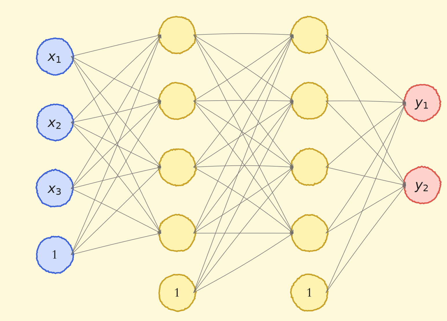
第1个隐藏层：使用Xavier正态分布初始化权重,激活函数使用Tanh。

第2个隐藏层：使用He正态分布初始化权重,激活函数使用ReLU。

输出层：按默认方式初始化,直接输出原始得分(logits),不在模型里套Softmax——原因紧接着代码说明。

import torch
import torch.nn as nn

class Model(nn.Module):
    # 初始化
    def __init__(self):
        super(Model, self).__init__()  # 调用父类初始化
        self.linear1 = nn.Linear(3, 4)  # 第1个隐藏层,3个输入,4个输出
        nn.init.xavier_normal_(self.linear1.weight)  # 初始化权重参数
        self.linear2 = nn.Linear(4, 4)  # 第2个隐藏层,4个输入,4个输出
        nn.init.kaiming_normal_(self.linear2.weight)  # 初始化权重参数
        self.out = nn.Linear(4, 2)  # 输出层,4个输入,2个输出,默认使用He均匀分布初始化

    # 前向传播
    def forward(self, x):
        x = self.linear1(x)  # 经过第1个隐藏层
        x = torch.tanh(x)  # 激活函数
        x = self.linear2(x)  # 经过第2个隐藏层
        x = torch.relu(x)  # 激活函数
        x = self.out(x)  # 经过输出层, 输出2维logits(未归一化的类别得分)
        return x

model = Model()
output = model(torch.randn(10, 3))
print("输出logits(尚未归一化为概率)：\n", output)
print("softmax之后才是概率：\n", torch.softmax(output, dim=1))
print()

# 使用named_parameters()查看各层参数
print("模型参数：")
for name, param in model.named_parameters():
    print(name, param)
    print()

# 使用state_dict()查看各层参数
print("模型参数：\n", model.state_dict())

这个自定义模型把今天的内容串成了完整闭环：__init__里搭结构、选初始化,forward里走前向——注意代码里没有写任何反向传播,autograd会自动搞定。初始化和激活函数的搭配也有讲究：Tanh配Xavier、ReLU配He,正是1.10节和1.11节讲的原则。输出层为什么不套Softmax？ 因为PyTorch的nn.CrossEntropyLoss内部已经包含了Softmax(且数值更稳定),模型里再套一遍就成了双重Softmax。训练时输出logits直接交给损失函数;只有在需要"看到概率"或做预测时,才像上面那样手动torch.softmax或取argmax——Day20会把这条规则再强调一次。

1.12.2 查看模型结构和参数数量

可使用torchsummary.summary来查看模型结构与参数数量。需要先安装torchsummary库：pip install torchsummary。

from torchsummary import summary

# input_size:特征数,batch_size:样本数
summary(model, input_size=(3,), batch_size=10, device="cpu")

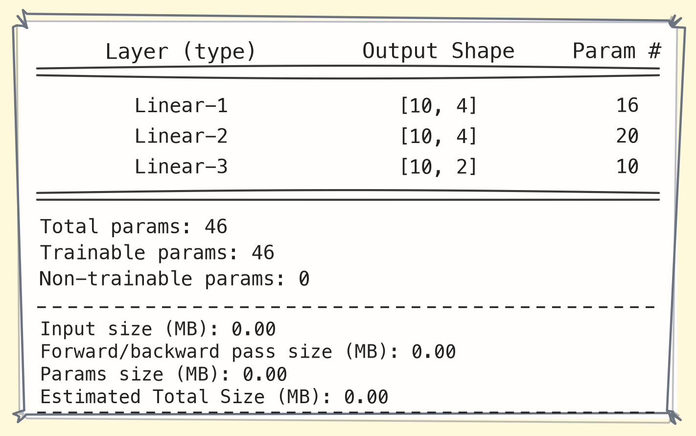
以第1个隐藏层为例：每个节点有3个权重与1个偏置,计4个参数,4个节点共计16个参数。

1.12.3 使用Sequential构建模型

可以通过torch.nn.Sequential来构建模型,将各层按顺序传入。

# 构建模型(输出层给logits, 不套Softmax——CrossEntropyLoss自带, 见1.10.1)
model = nn.Sequential(
    nn.Linear(3, 4),
    nn.Tanh(),
    nn.Linear(4, 4),
    nn.ReLU(),
    nn.Linear(4, 2),
)

# 初始化参数
def init_weights(m):
    # 对Linear层进行初始化
    if type(m) == nn.Linear:
        nn.init.xavier_uniform_(m.weight)
        m.bias.data.fill_(0.01)

model.apply(init_weights)  # apply会遍历所有子模块并依次调用函数

logits = model(torch.randn(10, 3))
print("输出logits：\n", logits)
print("需要概率时再手动softmax：\n", torch.softmax(logits, dim=1))

model.apply(init_weights)是个实用技巧：它会递归遍历所有子模块,对每个Linear层统一做初始化,不用一层层手写。

Sequential类使模型构造变得简单,不必自定义类就可以组合新的架构。然而并不是所有的架构都是简单的顺序架构,当需要更强的灵活性时还是需要自定义模型。比如ResNet的残差连接、多输入多输出的结构,Sequential就无能为力了。

小结

今天从张量操作走到自动微分,再到一个能跑的线性回归和完整网络,把PyTorch训练的核心零件备齐了：

• 张量是PyTorch的基本数据结构,创建、运算、索引、形状、拼接的API是后面所有代码的地基;送进GPU前要转成float32,autograd也只对浮点张量求导。
• autograd只管前向记图,backward()沿计算图自动求导,链式法则由框架替你跑;非叶子节点梯度反向后释放、叶子节点累积,所以每个batch要先zero_grad()。
• 训练循环三件套：zero_grad()→backward()→step(),顺序不能乱;推理和验证用torch.no_grad()或model.eval()关掉追踪和Dropout。
• **nn.Module**靠__init__注册子层、forward定义前向,调用时写model(x)而不是model.forward(x);参数由框架自动收进model.parameters()。
• 初始化与激活搭配：Tanh/Sigmoid配Xavier,ReLU一族配He;多分类输出层给logits、不套Softmax,交给nn.CrossEntropyLoss。

从Day18手推链式法则到今天用框架自动求导,训练链路已经成型。Day20会把autograd、nn.Module、损失函数和优化器组装成一条完整的训练链路,再从全连接层跨入卷积神经网络——守住图像的空间结构。